Casting Defect Inspection System, Raghav Singh

Visual inspection of cast parts is slow and inconsistent between operators, and a missed defect is expensive downstream. I wanted to see whether a single photo of a part could be turned into a reliable accept-or-reject call, with a visual the inspector could actually trust. I built the whole thing end to end: the data pipeline, the model, the explainability layer, and the dashboard it runs in.

What I built

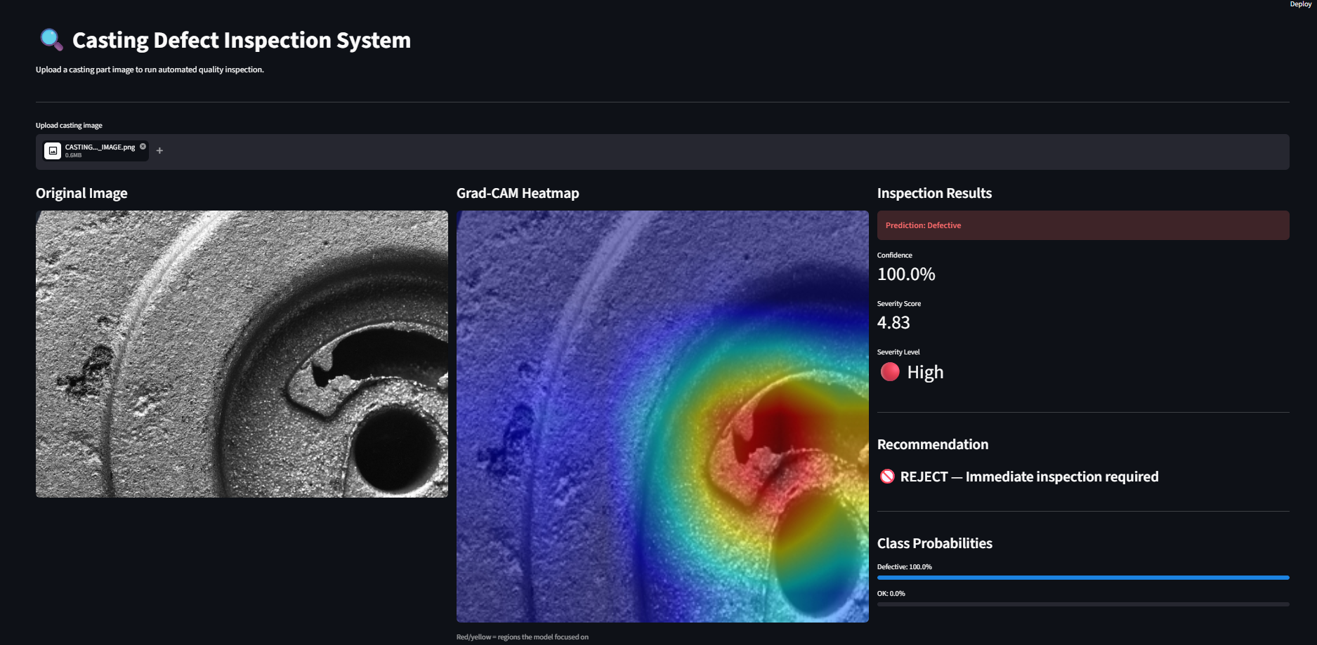
Everything, on my own. I assembled and cleaned the dataset, wrote the two-stage transfer-learning training in PyTorch, added Grad-CAM so each prediction shows what the model reacted to, and deployed it as a Streamlit dashboard that takes an image upload and returns a class, a confidence, and a disposition. Trained on Google Colab.

Inspection dashboard: original image, Grad-CAM heatmap, and results panel — FIG 1 · The dashboard. Left: input casting. Centre: Grad-CAM activation, concentrated on the surface flaw rather than the background or part edges. Right: class, confidence, and disposition.

Model data
Task	Binary classification, defective or acceptable
Dataset	7,000+ labeled cast-metal images (public)
Backbone	ResNet18, ImageNet pretrained
Training	Two-stage: frozen backbone, then unfrozen final block
Test accuracy	96%
Explainability	Grad-CAM class activation maps
Stack	Python · PyTorch · Streamlit · Colab (T4)

Design decisions

Transfer learning over training from scratch. 7,000 images is far too few to learn general edge and texture features, so the pretrained backbone supplies them and only the task-specific layers are fitted.
Two-stage fine-tuning. Training the head first with the backbone frozen prevents large early gradients from wrecking the pretrained weights. Unfreezing the final block afterwards adapts the highest-level features to cast surfaces.
Grad-CAM as the acceptance check. Accuracy alone doesn't show whether the model learned the defect or a lighting artifact. The heatmap confirms activation sits on the flaw, which is what makes the tool trustworthy to an inspector.

The classifier itself worked. The harder problem was grading how defective a part is, so borderline parts could be triaged instead of scrapped. That turned out to be the real engineering of the project, and it did not go the way I first expected.

Challenges

Severity scoring, three approaches that failed. I first tried to grade severity with classical image processing: Canny edge detection, adaptive thresholding, and local texture variance. None of them separated defective from acceptable reliably. The root cause is that this dataset's defects are subtle and varied, they don't produce a strong global signal, and there are no pixel-level defect labels to learn from. So the clean computer-vision approach simply wasn't available.
What I did instead, and its limits. I fell back to a baseline-deviation method: a z-score of each part against the distribution of healthy parts. It gives a weak but directional severity signal, enough to flag "clearly bad" from "borderline." I documented it honestly as a limitation rather than dressing it up, because a false sense of a precise severity number would be worse than none.
Training that wouldn't finish. My first Colab runs read images straight from Google Drive and the session disconnected before the first epoch finished. Copying the dataset into Colab's local storage first cut each epoch from over five minutes to one or two, and the runs completed.